How we migrated our data warehouse from Redshift to BigQuery

We recently migrated our data warehouse at Omio from AWS Redshift to Google BigQuery.

My team recently migrated our data warehouse at Omio from AWS Redshift to Google BigQuery.

There were several compelling reasons.

• The rest of our company’s infrastructure runs on Google Cloud. Our BI data pipelines were traditionally run on AWS for legacy reasons¹ and it was time for us to align with the rest of the organization.
• Redshift requires non trivial amount of effort to keep running. Although Redshift has improved quite a lot in this area (with concurrency scaling, elastic resize etc.), it is still not as hands-free as BigQuery.
• We found BigQuery performance to be orders of magnitude better than Redshift for our use cases. It is also much more forgiving of poorly written legacy code.
• Some teams (for ex. Marketing ) were already using BigQuery due to its deeper integration with Google Analytics and Adwords. Hence, it made sense to store all data in a single data warehouse.
• There were significant cost savings in using a single data warehouse instead of two.

Challenges

Our data pipelines have grown significantly in the last few years. But this has also created an unwanted amount of legacy code through our data infrastructure. Attempting a warehouse migration in this environment was tricky because

• There were a large number of tables and datasets to be migrated. We had over 150 tables across multiple schemas and almost an equal number of downstream systems and processes.
• Several core legacy pipelines (mostly batch jobs) were written purely in SQL over Redshift. These are poorly documented and very difficult to understand .
• Many internal teams consume the data from the warehouse using various tools (plain SQLs, Tableau, Redash and many more). It is difficult to keep track of all these users and the way they use data. A migration project meant communicating and getting support from all these teams and making it easy for them to quickly migrate.
• At the time when we started this project, we were forced to go fully remote due to the Covid-19 situation with the entire team on reduced working hours. This made it difficult to coordinate the various activities around this project.

Challenges notwithstanding, we were able to successfully complete the migration in two months. The remainder of this post describes our approach and learnings in detail.

Step-1: Copy the data

We decided that a key step in this process was to first move all the tables from Redshift to BigQuery in order to allow our end users to migrate their downstream jobs/queries seamlessly.

One of our engineering teams had earlier built an excellent tool in Golang called Blueshift to create incremental replicas of tables from Redshift to BigQuery. Blueshift takes a yaml configuration file with details of the source and destination tables and triggers a Google DataFlow job to copy data. Blueshift also watermarks the data it has copied - this enables it to copy data incrementally in subsequent runs.

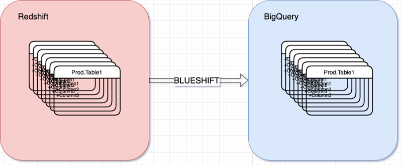
Since there were 100s of tables to be copied, we wrote another small Python tool called Shifty to automate the generation of Blueshift config files for all our tables. The copy jobs were orchestrated in Apache Airflow each morning when the latest data got updated in Redshift.This approach allowed us to make all the tables available in BigQuery even though our batch jobs were still running on Redshift.

Step-2: Migrate Data Pipelines

This is where the fun began. To migrate the batch jobs, we needed to port the SQL code from Redshift to BigQuery. This sounds easy but there are several differences between the SQL syntax and functions supported by Redshift and BigQuery. So each query needed to be carefully rewritten without breaking anything or introducing bugs.

Let’s take an example.

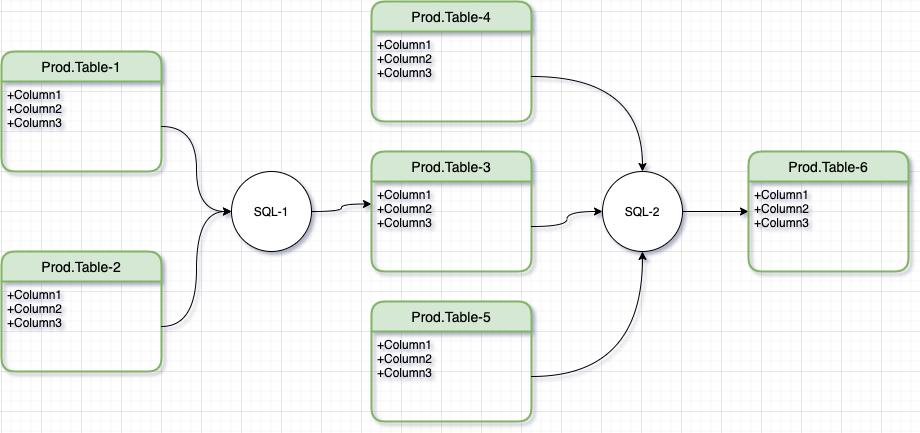Simple Batch Pipeline with 2 transformation steps

Let’s imagine a simple batch process with 2 transformation steps, SQL-1 and SQL-2. SQL-1 reads Table-1 and Table-2, transforms and writes the output to Table-3. The next step, SQL-2 then reads from Table-3, Table-4 and Table-5 and produces Table-6 as the final result².

Notice that in this pipeline, Tables 1,2,4 and 5 are read-only. Tables 3 and 6 are written (updated) by the transformation steps. This means that in order to test this pipeline, we need to test data in Tables 3 and 6 against expected values.

If you look closely, this pipeline can be interpreted as a chain of two functions

Each of these functions can be considered as a separate step that can be developed and tested in isolation. What’s more, these steps can be developed in parallel. Let’s see how.

Migrating each transformation step in isolation

For the first transformation step, SQL-1, we can proceed to rewrite it in BigQuery by reading its inputs, Table-1 and Table-2 from Production schema (which are copies of Redshift tables. See Step-1) and writing to a Development schema.

If the new output (Dev.Table-3) exactly matches it’s Redshift cousin (Prod.Table-3), then we can be confident that our migrated code in SQL-1 is working fine. This is exactly the idea behind characterization test as proposed by Michael Feathers and others as a way to safely change legacy code.

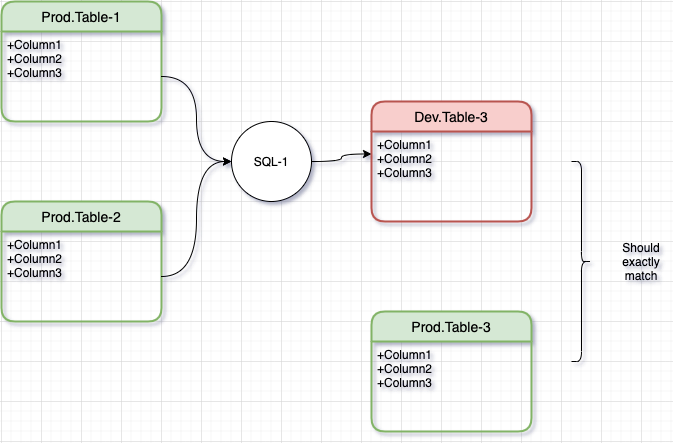
We decided to strictly adopt a lift and shift strategy in order to minimize the vector of change. This meant that we avoided the urge to refactor or optimize the SQL logic even in cases where we suspected it to be redundant or unoptimized. It was important that we focussed on one problem at a time.

Likewise, for the next step in the pipeline

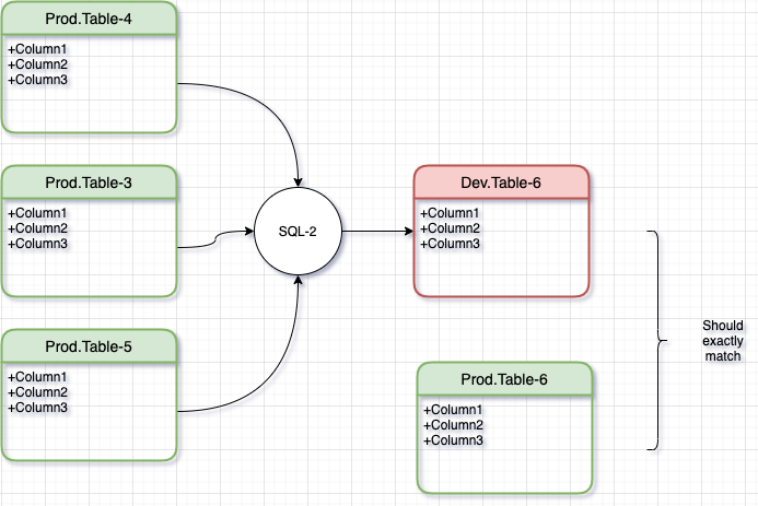
Notice here that for this step, Table3 is read-only and therefore we use Prod.Table3 and not Dev.Table-3. This is key in isolating these transformation steps so they can be unit tested.

By isolating the 2 steps this way, both can be developed and tested in parallel.

Integration Testing

Once the individual SQLs are unit-tested, it’s time to integrate them. Here, we connect them as follows

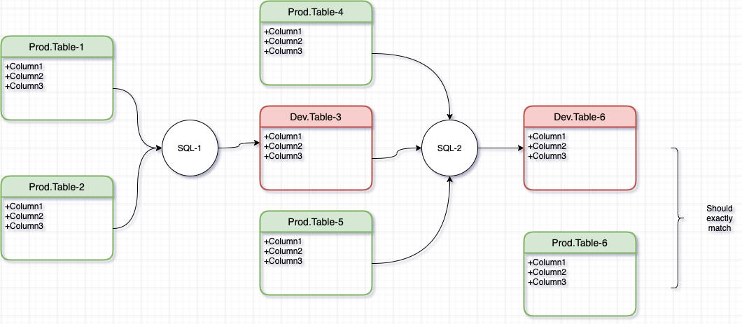
Notice again that this time, we are now using Dev.Table-3 as input to SQL-2. The final output of Dev.Table-6 should still be compared with the Prod version to make sure everything looks good.

At this point, if the new data exactly matches the Prod data, we are ready to replace Dev.* tables with Prod.* tables in the pipeline. The migration of this pipeline is complete.

Data Quality

To make sure we didn’t break anything in the migration process, thorough data testing was needed. We wrote a small tool in Python called wasserwaage ( German for a carpenter’s spirit level) which was essentially a wrapper around Python’s excellent datacompy module. This tool helped us compare snapshots of data between Prod and Dev tables and printed even the smallest differences that it found between two datasets.

It was also important to test our migrated pipeline for a certain period of time and continuously compare the output with the baseline. We relied on Redash for this and built a set of dashboards to compare daily aggregated metrics from the new pipelines with the corresponding production values.

Rollout

Since we had already copied the tables (Step-1), we were able to simply replace these copies with the new versions in production without impacting downstream users³ as soon as an ETL was ready to be deployed. This allowed us to continuously rollout finished ETL jobs whenever they were ready.

Additional Notes

• We use Apache Airflow for our batch pipelines. We have an excellent CI/CD setup that allowed us to integrate and test the pipelines very fast.
• We decided to cut down on the process overheads and switched from Scrum to Kanban during the migration project. We normally follow a two week sprint but the nature of this project and the Kurzarbeit situation compelled us to adopt a less ceremonious process⁴.
• Our Apache Spark based pipelines (batch and streaming) were relatively easier to migrate although they had their own challenges (build-deploy-run feedback loop for Spark jobs is usually slower compared to SQL)
• We over-communicated on Slack to offset the limitations posed by remote working.

Key Takeaways

• In the first step, we moved our tables so end-users of data could immediately migrate. This helped us achieve very high productivity as teams could work in parallel.
• We decided to not change any table contracts so teams could migrate their queries and dashboards easily.
• We prioritized migrating the most complex pipelines first. This allowed us to learn early and gain confidence faster. The less complex pipelines felt like a breeze once the steepest mountains were climbed.
• We adopted a Lift and Shift approach to minimize the change vectors. This helped us remain focussed on the migration without getting distracted by irrelevant changes.
• We isolated units of pipeline and tested them independently using characterization tests. This gave a massive boost to our productivity as we could work in parallel on different parts of the pipeline.
• We automated the boring steps to further speed up the process.
• We tailored our agile process to reduce process ceremonies.

---

Footnotes

1. Snowplow, our main tracking system, only supported AWS when the core BI pipelines were created.
2. This, of course, is a simplification and in reality, a typical data pipeline has several such steps with multiple complex joins and transformations.
3. That’s why it was important to not change the contracts (i.e. DDL) of the migrated tables.
4. Once the scope was defined, we created a list of jobs to be migrated and assigned them to the team. We felt that a simple Kanban board was a more efficient way to track the project and some of the usual sprint ceremonies (sprint planning, review etc.) could be cut down.